Nonparametric Kernel Density, Nonparametric Regression and Binary-Choice Models.
The data set used in this assignment comes from Pindyck and Rubinfeld (1998) “Econometric Models and Economic Forecasts” and contains the following variables: a dummy whether children attend private school (private), number of years the family has been at the present residence (years), log of property tax (logptax), log of income (loginc), and whether one voted for an increase in property taxes (vote). There are two dependent variables of interest -private and vote- which can be modeled individually by two univariate probit models or jointly by one bivariate probit model, for instance.
Link to PDF HERE.
Binary Choice Models
Kernel Density Estimation
Before running a binary choice model to explain the voting choice, we plot different Kernel Density estimates of loginc to check whether it follows approximately a normal distribution. The idea is to test visually if the normal distribution falls within the 95% confidence interval area of each kernel density estimate:
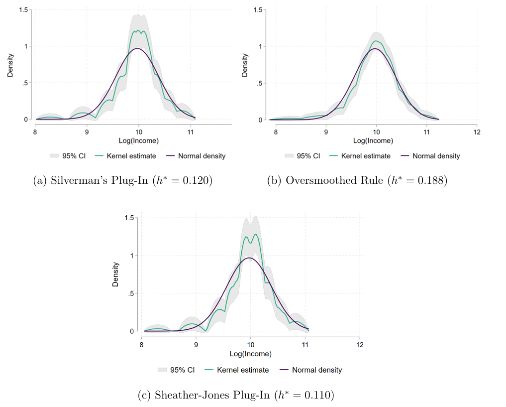
All these Kernel Density estimators in Figure 1 use an alternative Epanechnikov Kernel function (this is the default in the kdens command in STATA). The differences among the estimator are explained by the different methods of choosing the Optimal Bandwidth \(h^*\) that minimizes the Mean Integrated Squared Errors (MISE)1. Comparing the kernel densities of the log income against the normal distribution, we observe that the normal distribution seems to not quite fit inside the confidence intervals in none of the kernel estimators. While the case of an optimal bandwidth of \(h^*=0.188\) in Figure 1.b. seems to present some evidence about normality, you can still see how the purple line appears outside the boundaries around the 9 to 9.5 value.
Both Plug-in methods (Figure 1.a. and 1.c.) use a lower Optimal Bandwidth (0.11 and 0.12, respectively), thus, leading to less bias but more variance in their estimates. In these cases, the normal distribution line appears outside the 95% confidence boundaries in several places. Overall, the visual test seems to reject the hypothesis that log incomes follow a normal distribution.
Binary Choice Model (probit)
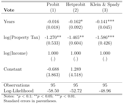
Table 1 reports the results of different Binary choice models to predict voting behavior using years, logptax and loginc as independent variables:
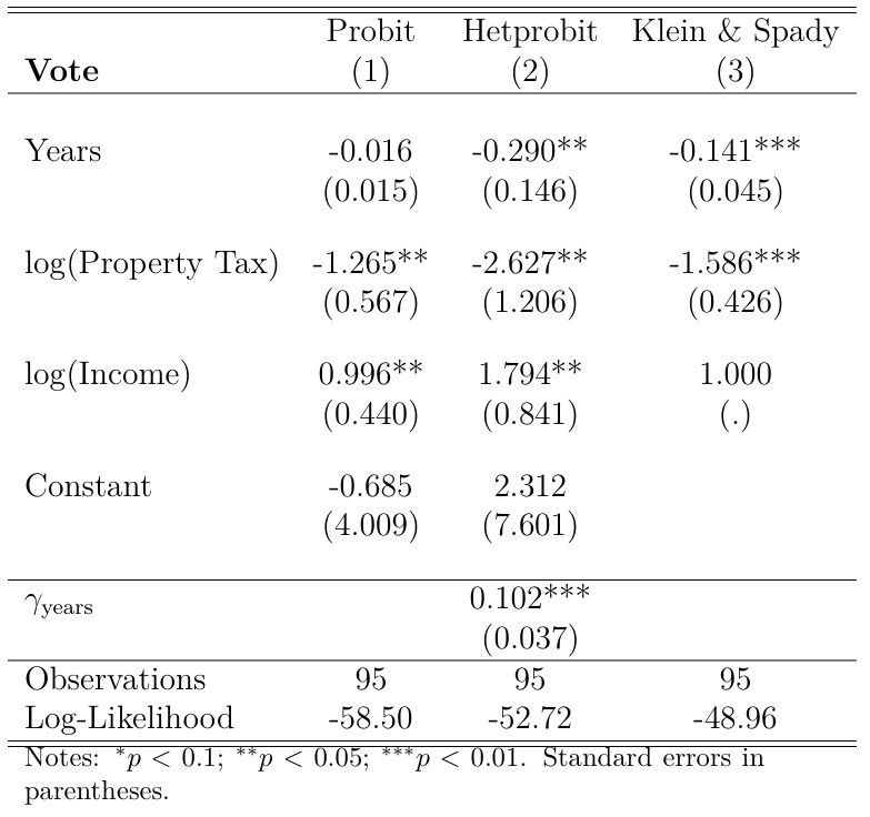
Column 1 in Table 1 presents the results of the probit model. Here we see a positive and statistically significant relationship between the level of log income and the probability of voting for higher property taxes. Also, once again we observe that property taxes have a negative effect on voting in favor of higher taxes of this kind. Finally, the number of years in the residence did not report a significant result.
Normality Assumption
We can use a visual test to check the normality assumption of the probit model estimated in Column 1. Recall that in the probit model, the probability that \(y_i\) takes on the value 1 is modeled as a nonlinear function of a linear combination of a set of independent variables:
\[ \Pr(y_i=1|x_i) = \Phi(x_i'\beta) \]
where \(\Phi(\cdot)\) is assumed to be the standard normal cumulative distribution function (CDF). To check if this assumption is reasonable, we performed nonparametric estimations of \(\Pr(y_i=1|x_{i'\beta})\). The first estimator is a Nadaraya-Watson Regression (or constant constant estimator) that assumes a constant \(m(x)=b_0(x_0)\) around some neighborhood of \(x_0\):
\[ \hat{m}_h(x_0)=\frac{\sum^N_{i=1} K_x\left(\frac{x_0-x_i}{h} \right)}{\sum^N_{i=1} K_x\left(\frac{x_0-x_j}{h} \right)}y_i \]
The Nadaraya-Watson estimator is essentially a weighted local average of the observations (weights defined by a Kernel function) at some neighborhood defined by the choice of bandwidth \(h\). The second estimator is a Local Linear Regression that, instead of assuming a constant average, lets \(m(x)\) be linear in the neighborhood of \(x_0\). More concretely, the local linear regression minimizes with respect to \(b_0(x_0)\) and \(b_1(x_0)\):
\[ \sum^N_{i=1} K_x\left(\frac{x_i-x_0}{h} \right)[y_i-b_0(x_0)-b_1(x_0)(x_i-x_0)]^2 \]
Both nonparametric regressions use the Epanechnikov Kernel function. Regarding the choice of bandw
idth \(h^*\), I use the command npregress that performs the Leave-One-Out Cross Validation method (LOOCV) to estimate the Optimal Bandwidth size2. Figure 2 compares these regressions against the probit estimation:
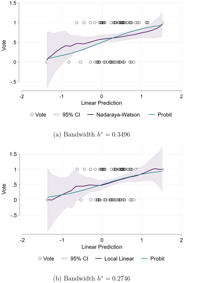
In general, we see that the normality assumption about the error term \(\varepsilon_i\) in the probit model is actually not rejected, as the probit curve of the \(\Pr(y_i=1|x_i'\beta)\) tends to be within the 95% confidence intervals of both the Local Constant and Local Linear nonparametric estimators. This means that the standard probit model does not suffer from misspecification.
Heteroscedastic Probit Model
Column 2 of Table 2 presents the results of the heteroscedastic probit model. This specification still assumes that the error term of the latent model follows a normal distribution, but is more flexible in the sense that it no longer assumes its variance to be 1, but that it can vary as a function of some set of explanatory variables. In this case, we only use the variable years to model the variance:
\[ V(\varepsilon_i|x_i)=\sigma^2_i=[\exp(\text{years}_{i}'\gamma)]^2 \]
where \(\varepsilon_i\sim N[0,\exp(\text{years}_{i}'\gamma)]\). The probability of success is now represented by:
\[ \Pr(y_i=1|x_i) = \Phi\left( \frac{x_i'\beta}{\sigma_i} \right) = \Phi\left( \frac{x_i'\beta}{\exp(\text{years}_{i}'\gamma)} \right) \]
Here we are primarily interested in testing whether \(\gamma\neq 0\), which seems to be the case as we see in Table 2 a statistically significant coefficient. Additionally, the likelihood-ratio test of heteroskedasticity, which tests the full model with heteroskedasticity against the full model without, is significant as \(\chi^2(1) = 11.55\). Regarding the coefficients, we now see that the number of years in the residence impacts negatively the probability of voting for higher property taxes. The remaining variables are still significant and with the same sign relative to the standard probit model, but the coefficients are more pronounced.
Nonparametric Regression
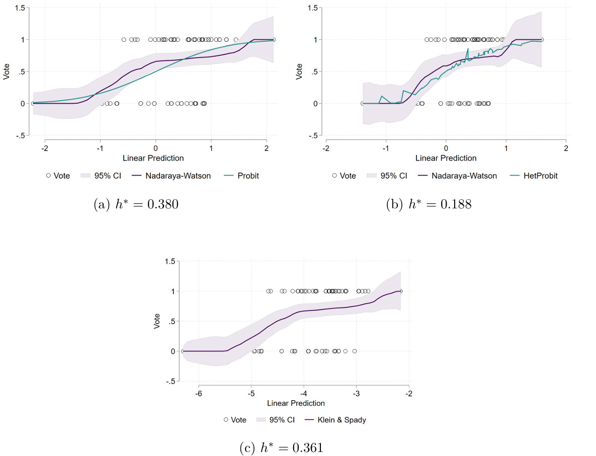
We now test again the normality assumption of the heteroscedastic probit model by visually comparing its CDF with the two nonparametric alternatives already discussed:
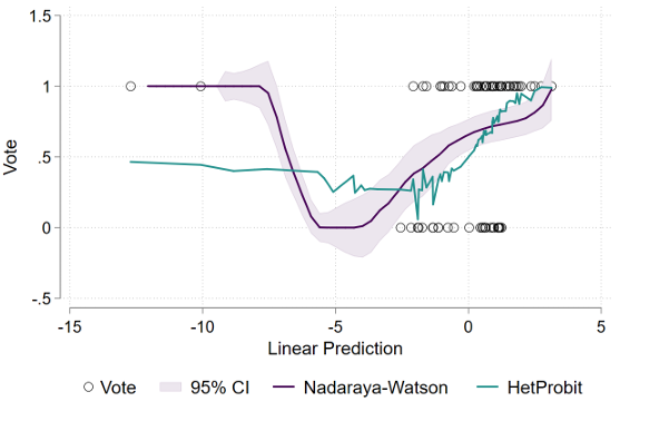
Clearly, the heteroscedastic alternative -that assumes normality- highly deviates from both nonparametric estimations. Hence, it seems that the normality assumption in the hetprobit model is rejected. Furthermore, the probit link function is no longer smooth when compared to the standard probit. Modeling the variance as dependent on the explanatory variable years makes the prediction less linear, leading to a more noisy curve than smoothed.
Klein & Spady Semiparametric Regression
Semiparametric alternatives do not rely on the parametric assumptions about the shape of the error term distribution \(\varepsilon_i\). The Klein & Spady method is a Single Index model with a \(\Pr(y_i|x_i)= F(x_i'\beta)\) structure that only depends on \(x_i\) through a single linear combination, \(x_i'\beta\), whereas the function \(F(\cdot)\) is left unspecified. The estimation is based on some kind of Maximum Likelihood Estimation:
\[ L(\beta,h)=\sum^N_{i=1}(1-y_i)\ln[1-\hat{F}_{-i,n}(x_i'\beta)]+\sum^N_{i=1}y_i\ln[\hat{F}_{-i,n}(x_i'\beta)] \]
Since \(F(\cdot)\) is unknown, Klein & Spady suggest replacing it with a Leave-One-Out Nadaraya-Watson estimator \(\hat{F}_{-i,n}(\cdot)\). In order to guarantee point identification, the coefficient of one continuous variable is normalized to 1, which in our case will be the variable loginc. Additionally, in single index models, the function \(F(\cdot)\) will include any location and level shift, so the vector \(x_i\) cannot include an intercept. Column 3 of Table 2 shows the results of this semiparametric regression. But because we want to make some comparisons between the different models so far presented, we will also need to scale normalize the previous models, as in Table 2 they are not directly comparable. Table 3 shows the results of each model after scale normalization:
Here we see that the direction of the signs in every specification is the same: years and logptax are negatively associated with the probability of voting in favor of the tax reform. The coefficients of the property tax variable are to some degree similar across models, but there are important differences regarding the coefficient linked to the number of years in residence. First, the probit model did not show an effect statistically distinct from zero, whereas the other two models did show significant and more pronounced coefficients.
Between the heteroscedastic probit and the Klein & Spady regression, the hetprobit seems to report a more negative effect of years on the probability of voting for higher taxes. In order to understand the magnitude of these differences between models, we will need to estimate marginal effects.
Semiparametric Regression Visualization
Figure 4 visualize the Klein & Spady semiparametric estimate of \(\Pr(y_i=1|x_i'\beta)\) and compares it against the heteroskedastic estimation:
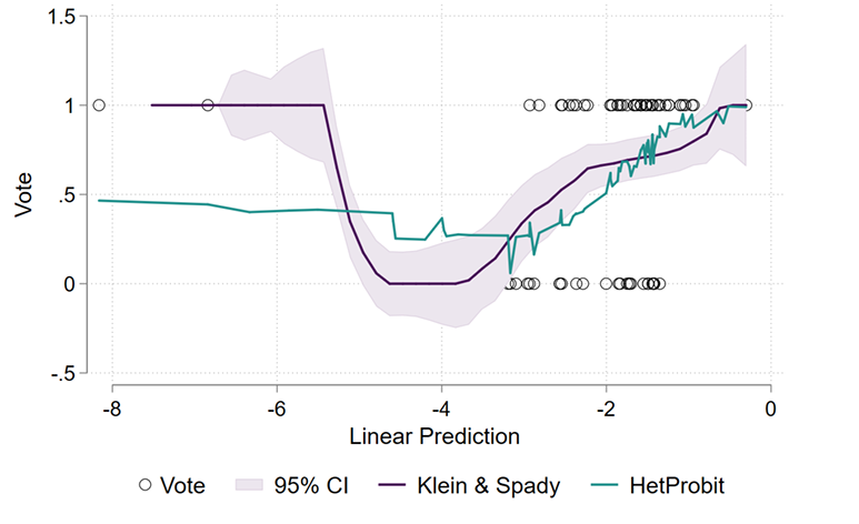
The semiparametric regression in Figure 4 this case is quite similar to the ``U’’ shape of the nonparametric (Nadara-Watson) regression from Figure 3.a. that is based on the predicted values \(x_i'\beta\) of the heteroscedastic probit to estimate the probabilities. However, we also see that the (parametric) heteroscedastic probit falls outside the 95% confidence interval area at various points ( Figure 4 in green). Hence, while we cannot use the hetprobit model to draw conclusions on the probability of voting for higher property taxes, we do can use a nonparametric version of the predicted values of the heteroscedastic model for that purposes.
Most of the behavior behind this strange shape of the link function -behavior that is mostly happening at \(x_i'\beta<-5\) in Figure 4 -, can be explained by the distribution of the years variable. From Figure 5 we can observe that this group consists of 5 observations that have an average number of years of 39, versus the 6.8 from the rest of the sample:
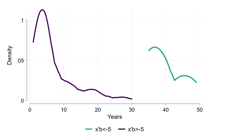
As we have seen from the models, the number of years has in general a negative effect on the probability of voting for more taxes, but here we have that all these 5 observations have a high number of years in the residence and all of them have vote=1. Hence, this group of ``outliers’’ might be generating a countervailing effect on the true point estimates of years.
Restricted Model
We now re-run the binary choice models so far discussed, but restricting the estimation for observations where the number of years in residence is smaller than 25. Table 4 shows the main results after normalization to make them comparable:
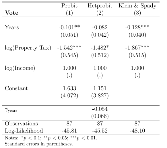
Here we see surprisingly similar conclusions on the point estimates across different specifications. In the standard probit model, we now see that years have statistically significant results, with a more intense negative effect on our dependent variable than before. The heteroscedastic probit now reports a more negative coefficient on the variable logptax, significant only at the 10% level, but for the number of years, we see a less pronounced effect and is no longer significant. Looking at \(\gamma\), note that now we cannot reject the null hypothesis of homoscedastic errors so that, after filtering for the extreme values of years, there is no evidence of this model being better than the standard probit.
Finally, the semiparametric model seems to be the model that changed the least. Both the direction of the signs and their significance remain as before, with years having a slightly less pronounced coefficient, and logptax reporting now a more negative effect on the probability of voting for higher taxes than before.
We want now to test the normality assumption, so we re-estimate the nonparametric regressions from previous exercises to make the visual comparison. In this case, I only perform the Nadaraya-Watson Estimator:
Again, we see that all both the probit and hetprobit models falls within the boundaries of the confidence interval of the nonparametric estimates. Taking all this evidence together, we can conclude that, after filtering the extreme values of years, the three binary choice models are no longer much different from each other. Finally, because now there is no evidence of heteroscedasticity and we did not reject the normality assumption about the error terms \(\varepsilon_i\), the standard probit model is the preferred model in my view.
Nonparametric and Semiparametric Regression Comparison
Using the standard probit estimates, we want now to graphically compare the estimates between the Nadaraya-Watson (Local Constant), the Local Linear, and the Local Quadratic regression. The following figure summarizes the results:
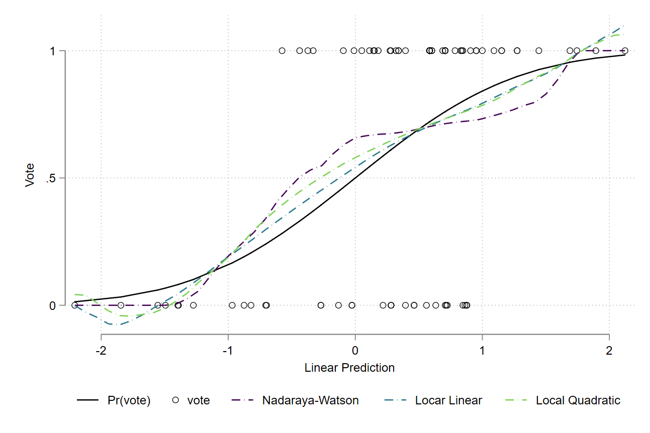
Although the curves seem to be very similar, we can identify some differences at specific points. Generally speaking, the degree of bias of the Nadaraya-Watson highly depends on the curvature or second derivative \(m''(x)\) of the regression function, as well on the slope of the density of the regressors \(f'(x)\):
\[ \text{bias}[\hat{m}(x)]=\frac{h^2\mu_2}{2}\left\{m''(x)+2\frac{f'_x(x)m'(x)}{f_x(x)} \right\}+O(\frac{1}{nh})+o(h^2) \]
Namely, the bias will be very large at a point where the density function curves a lot. In Figure 7 (and assuming the normality distribution is the true function), we can actually observe that the Local Constant estimator has a large and positive bias (i) between \(-1<x_i'\beta<0.5\), which is the place where the density is curving positively and very quickly (positive curvature) and (ii) between \(0.5<x_i'\beta<1.55\), marking the space where the density function is decreasing quickly (negative curvature). The local linear and local quadratic regressions also present this described behavior, but with less biasedness. The local linear is the more smoothed function among the three.
One reason that explains this difference may be due to the fact that the bias of the Local Linear (and Quadratic) regression does not depend on the density function of the regressors, also called design bias:
\[\begin{align*} \text{bias}[\hat{m}(x)]=\frac{h^2\mu_2}{2}m''(x)+o(h^2) \end{align*}\]
In that sense, the design bias adds an extra bias to the Nadaraya-Watson estimator. Finally, we observe more differences between the estimators on the extremes. On the bottom left (between -1.2 and -2), for example, the Nadaraya-Watson starts with higher bias, but then it shifts quickly to be equal to 0 towards the left, whereas the other two (which are very similar to each other) start with less bias, but then they end up with negative probabilities towards the left. On the other extreme we find the same behavior, where the local and quadratic estimators are not bounded to be within 0 and 1.
Footnotes
As the optimal bandwidth formula also depends on the curvature of the density \(f''\), which is unknown, there are different ways to deal with this issue. Some impose assumptions about the unknown distribution (Plug-in methods), and others are more data-driven such as cross-validation techniques.↩︎
In contrast, the command
lpolyuses the Rule-of-Thumb method of bandwidth selection, which is a Plug-In estimator.↩︎